
You've probably already compared two investments by looking at their announced returns. 5% for a euro-denominated fund, 8% for a World ETF, maybe 12% for USDC staking. But here's the problem: these figures tell you nothing about the timing of cash flows, actual fees, or the time value of money. An investment that pays 10% at the end of year five is not the same as one that pays 2% every year. To settle the question, you need two metrics that every financial analyst knows: NPV (Net Present Value) and IRR (Internal Rate of Return).
The problem is that Excel or Google Sheets aren't always enough. Either because you want to automate calculations across dozens of scenarios, or because you prefer to keep sensitive data off the cloud. The good news is that with about fifty lines of Python and zero external libraries, you can calculate both metrics yourself. I'll show you how to use NPV and IRR in Python with concrete examples drawn from real wealth management situations.
Why NPV IRR calculation in Python is essential for comparing your investments
Imagine two investment opportunities. First: you invest €50,000 in a life insurance contract with unit-linked funds promising a single payment of €68,000 in five years. Second: you invest the same amount in a staking protocol that pays you €4,000 per year for five years, then you get your capital back. Which one should you choose?
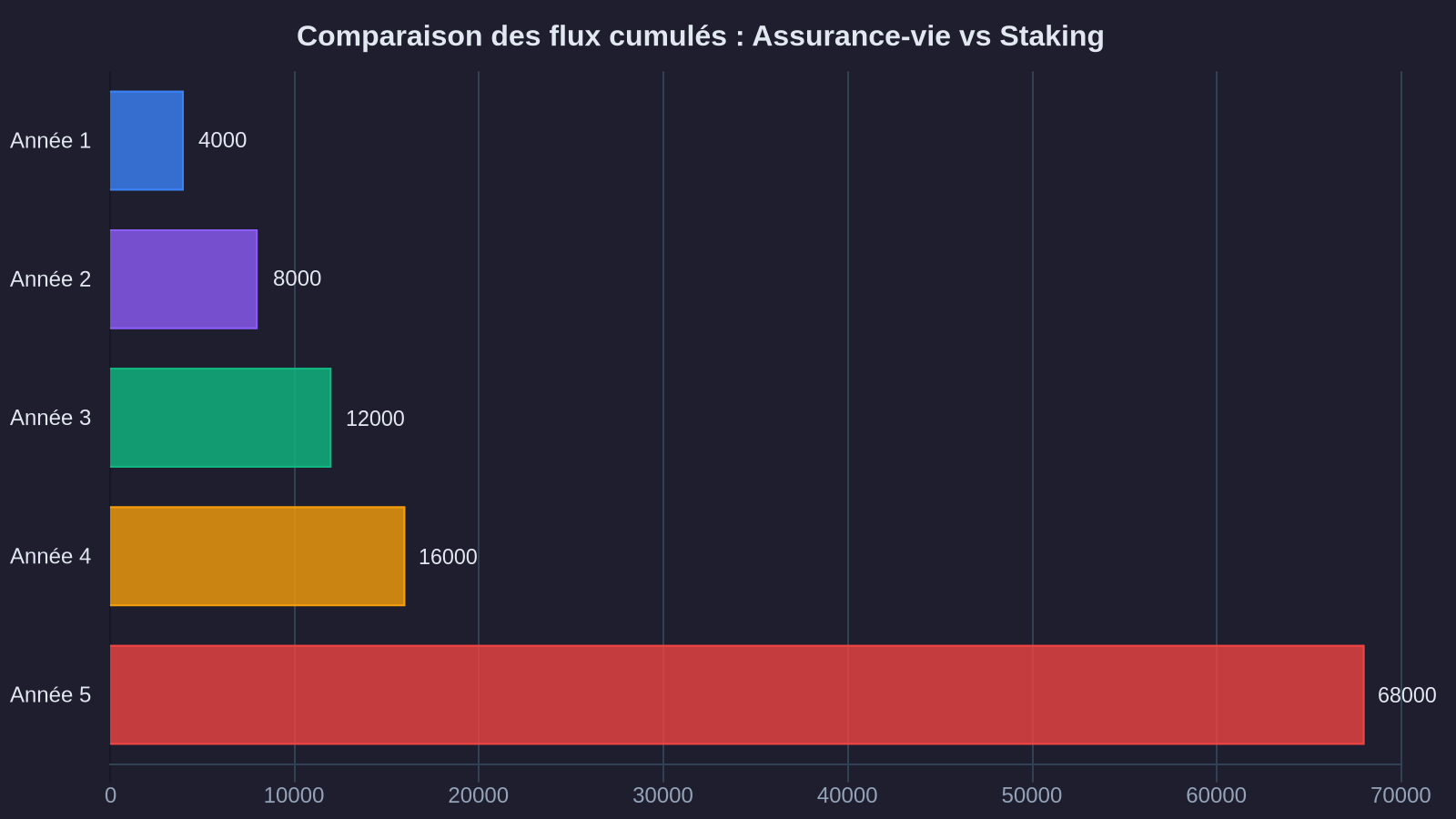
If you compare only the raw amounts, the first option yields €18,000, the second €20,000. But this comparison ignores a fundamental principle: a euro today is worth more than a euro tomorrow. Why? Because today's euro can be invested and generate interest. This is where NPV calculation in Python comes in.
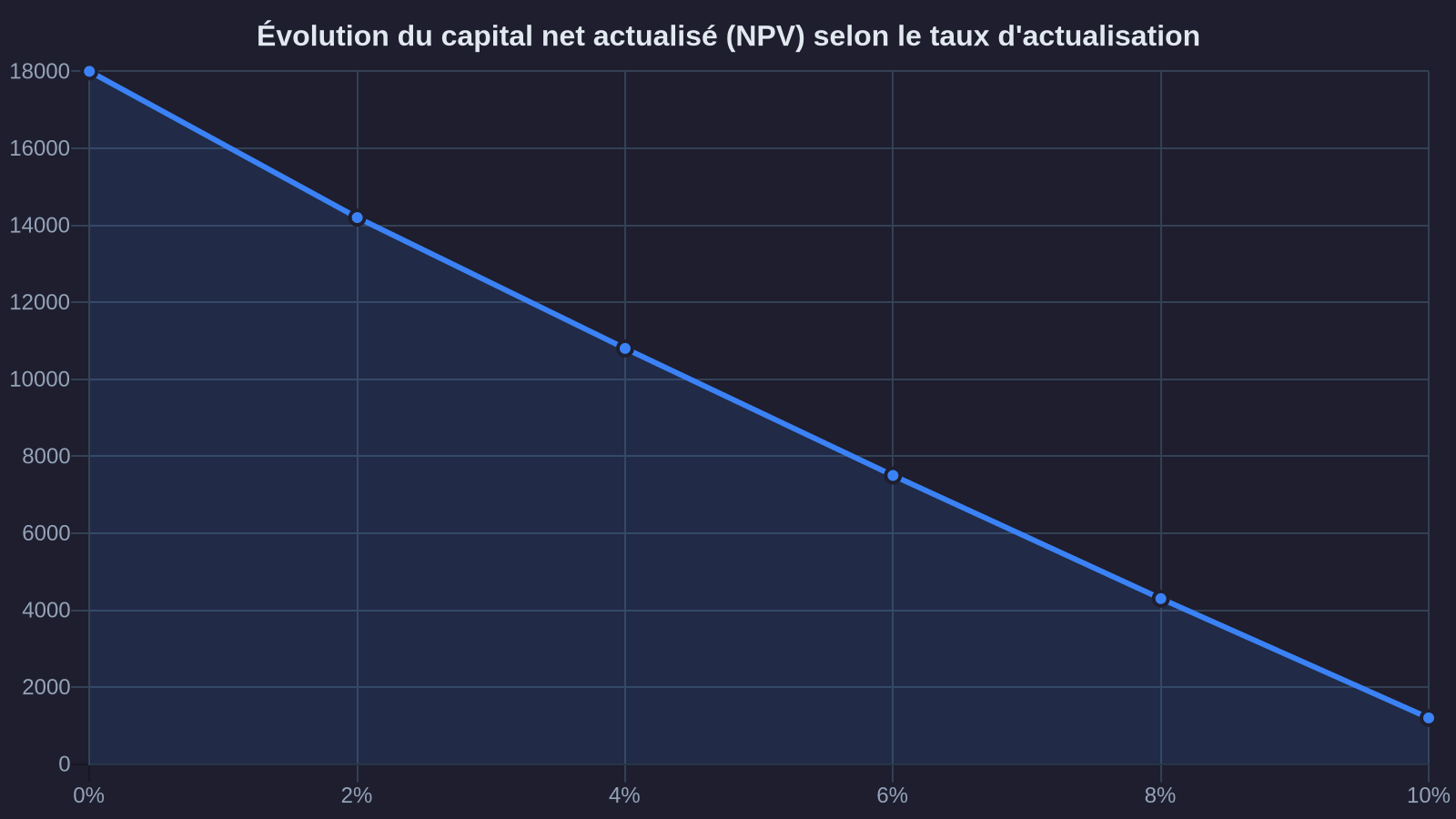
Net present value brings all future cash flows back to their value today by applying a discount rate. This rate represents the minimum return you require to accept locking up your capital. If your alternative is a savings account at 3%, your discount rate can't be lower. If you're targeting 6% net, that's your benchmark rate.
Take a concrete example. You invest €100,000 in an investment that pays you €5,000 per year for four years, then you recover €110,000 in the fifth year. If your discount rate is 4%, the NPV of this investment is €11,267. This means that, brought back to today, this investment is worth €111,267. In other words, it creates value relative to your return requirements.
IRR, on the other hand, answers a different question: what is the effective return rate of this investment? It's the rate that nullifies the NPV, the one at which the present value of future cash flows exactly equals your initial investment. In the example above, the IRR is 6.4%. You can then directly compare this 6.4% to the return of other investments: if your alternative yields 5%, the investment is attractive. If it yields 8%, you need to reconsider.
Coding NPV and IRR in Python: the mathematical fundamentals
The NPV formula is straightforward on paper. For each future cash flow, you divide it by (1 + rate)^n, where n is the number of years. You sum all these discounted flows and subtract the initial investment. NPV calculation in Python boils down to a function of just a few lines.
Here's a minimal implementation:
def npv(rate, cash_flows):
    total = 0
    for i, flow in enumerate(cash_flows):
        total += flow / ((1 + rate) ** i)
    return total
This function takes two parameters: rate, the discount rate (expressed as a decimal, so 0.05 for 5%), and cash_flows, a list that starts with the initial investment (negative amount) followed by all future cash flows. For example, for an investment of €50,000 that yields €3,000 per year for three years then repays the capital, you would pass [-50000, 3000, 3000, 53000].
IRR is trickier. There's no direct algebraic formula to calculate it; you have to use successive iterations. The idea: you search for the rate at which NPV equals zero. You start with an estimate (for example 10%), calculate the NPV, then adjust the rate based on the result. This is the Newton-Raphson method, which converges quickly in most cases.
Here's a working implementation to calculate IRR in Python:
def irr(cash_flows, iterations=100, tolerance=1e-6):
    rate = 0.1
    for _ in range(iterations):
        npv_value = npv(rate, cash_flows)
        if abs(npv_value) < tolerance:
            return rate
        derivative = sum(-i * flow / ((1 + rate) ** (i + 1)) for i, flow in enumerate(cash_flows))
        rate -= npv_value / derivative
    return rate
This function calculates the derivative of NPV (necessary for Newton-Raphson), then adjusts the rate until NPV is close enough to zero. In practice, this rarely takes more than ten iterations. The tolerance parameter defines the desired precision: 1e-6 means you accept a margin of error of one millionth, which is plenty for wealth management decisions.
Concrete examples of financial analysis in Python: crypto, real estate, and life insurance
Let's look at three typical wealth management situations and see how NPV and IRR help you decide.
Calculating investment returns: USDC staking vs euro funds
You're torn between investing €100,000 in a euro fund at 3% guaranteed, or in a USDC staking protocol at 8% (variable return, smart contract risk). With the euro fund, you get €103,000 each year, which you reinvest. With staking, you withdraw €8,000 annually, convert it to euros and spend it, then recover your capital after five years.
Euro fund cash flows (capitalized): [-100000, 0, 0, 0, 0, 115927]
USDC staking cash flows: [-100000, 8000, 8000, 8000, 8000, 108000]
With a discount rate of 4% (your minimum requirement), the NPV of the euro fund is €14,231. That of staking is €20,467. The IRR of the euro fund is 3% (makes sense, it's the guaranteed return), that of staking is 8%. On paper, staking wins. But be careful: this 8% is expressed in USDC, not euros. If USDC loses its peg or if the protocol suffers an exploit, your real IRR collapses. This is where wealth management judgment takes back the reins.
Buying real estate with anticipated resale
You buy a rental apartment for €250,000, notary fees included. You rent it for €1,200 per month (€14,400 per year after expenses), and anticipate a resale at €280,000 in seven years. You want to know if this project beats an REIT at 4.5% net.
Cash flows: [-250000, 14400, 14400, 14400, 14400, 14400, 14400, 294400]
With a discount rate of 4.5%, the NPV is €12,863. The IRR is 5.1%. This is slightly higher than the REIT, but you need to factor in taxation (income tax on rental income, capital gains), management, and rental risk. If you discount at 6% to account for these constraints, NPV becomes negative. Direct real estate is then no longer competitive.
Portfolio evaluation: choosing between life insurance and equity savings accounts with scheduled contributions
You're torn between contributing €500 per month for ten years to a life insurance policy (expected return: 4% net after management fees) or to an equity savings account invested in ETFs (expected return: 6% pre-tax, or about 5.3% after flat tax on exit).
With life insurance, you invest €60,000 total (€500 × 12 × 10). With a 4% return, you recover approximately €73,400 after ten years.
With the equity savings account, at 5.3% net, you recover approximately €77,600.
Life insurance cash flows: [-500 per month capitalized] → simplify to annual flows: [-6000, -6000, ..., 73400]
Equity savings account cash flows: same, with 77600 on exit.
The IRR of the equity savings account is 5.3%, that of life insurance is 4%. But life insurance offers an annuity option, advantageous tax treatment on inheritance after age 70, and the option for partial withdrawals without losing the seniority status. These are benefits that IRR doesn't capture. This is why these tools are decision aids, not oracles.
The limitations of NPV and IRR: what they don't tell you
These metrics are powerful, but they have blind spots. NPV assumes you can reinvest intermediate cash flows at the chosen discount rate. If you withdraw €5,000 per year from an investment and spend it, NPV overestimates the value creation. IRR, meanwhile, assumes you reinvest at the IRR rate itself, which is often unrealistic.
Another limitation: these calculations ignore volatility. A crypto investment showing a 15% IRR but whose value fluctuates 40% during the year doesn't have the same risk profile as a stable 5% bond. NPV doesn't capture your risk tolerance or liquidity needs. If you have to sell urgently at -30% because of an emergency, your theoretical IRR won't help you.
Finally, beware of overly optimistic projections. A staking opportunity at 20% that assumes protocol stability over five years is a fragile hypothesis. A property resold 30% higher in ten years is possible, but not guaranteed. NPV and IRR are only as good as your initial assumptions. Garbage in, garbage out.
What this means for your wealth
Calculating NPV and IRR yourself with Python, without relying on Excel or an advisor, means taking control of your decisions. You can test ten scenarios in two minutes, adjust assumptions, compare heterogeneous investments (crypto, real estate, structured products) on a common basis. You move beyond marketing claims and announced returns to enter actuarial reality.
But these tools don't replace judgment. An 8% IRR on an illiquid, risky investment isn't equivalent to a 6% IRR on a guaranteed fund. Taxation, liquidity, volatility, your investment horizon: all of this must weigh in the balance. NPV and IRR calculation in Python tells you how much value an investment creates. It's up to you to decide whether that value justifies the risk taken.
Your wealth deserves better than a savings account. I'm showing you the way, with numbers to back it up.